Introduction
The end goal for a professional investment consultant is to optimize risk-adjusted performance, otherwise known as maximizing the tradeoff between risk and return on the efficient frontier. To accomplish this quantitatively, an asset allocation model is run to determine the optimal asset mix. Portfolio construction requires the knowledge of modeling security returns, risks and their relationships.
Prices
The change of a security's price is generally affected by four factors, shown below with examples of their corresponding data components. A factor's influence is reflected by the steady or sudden increase or decrease in the price of the security.
| Factor | Examples |
|---|---|
| Fundamental Information | Company reported earnings, earnings estimates, industry reports, corporate debt, fraud, corporate cash flow, etc. |
| Economic Environment | Soureign default risk, interest rate changes, Federal Reserve policy, currency issues, unemployment rates, political regimes, etc. |
| Investor Psychology | Sentiment changes, fear & greed, bullish & bearish, beliefs, risk aversion, etc. |
| Technical Analysis | RSI indicators, MACD crossover, moving-averages, Point & Figure, etc. |
Returns
Financial Returns
Return is defined as the percentage gain or loss of a financial asset in a given time interval. The daily rise and fall of a security's price creates fluctuations in the daily return. A simplified example of this process is shown below.
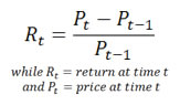
The mathematical formula to determine the return on an invested amount can be written as Rt = (Pt - Pt-1) / Pt-1 where R is the return, P is the price, and t is the time increment to be used (hours, days, weeks, etc.)
It states that to find the return for any day (t), subtract the previous day (t-1) amount (P) from that day's amount, then divide by the previous day's amount. The table below shows the daily return on a $100 asset purchase where the price of the asset increases $1.00 each day.
| Day | Price | Formula | Daily Return |
|---|---|---|---|
| 1 | $100 | ||
| 2 | $101 | (Day 2 P - Day 1 P) ÷ Day 1 P = ($101-$100) ÷ $100 | 1.00% |
| 3 | $102 | (Day 3 P - Day 2 P) ÷ Day 2 P = ($102-$101) ÷ $101 | 0.99% |
| 4 | $103 | (Day 4 P - Day 3 P) ÷ Day 3 P = ($103-$102) ÷ $102 | 0.98% |
| 5 | $104 | (Day 5 P - Day 4 P) ÷ Day 4 P = ($104-$103) ÷ $103 | 0.97% |
| 6 | $105 | (Day 6 P - Day 5 P) ÷ Day 5 P = ($105-$104) ÷ $104 | 0.96% |
Assuming no dividends, the simple return of a financial asset over the holding period from time t — 1 to time t is defined as:
The log return , also called a continuously compounded return, is defined as:
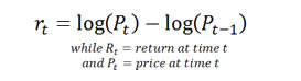
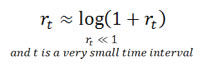
If rt is small, the log returns are approximately equal to simple returns
Return Distribution
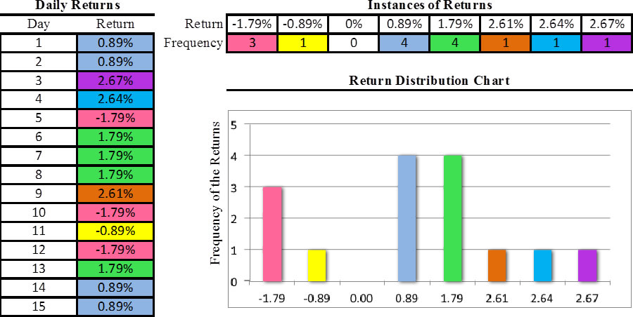
Over several equal intervals, returns within that period are calculated by the method mentioned previously and stacked up by their frequency, which forms a return distribution. Here is an extremely simplified example of how an empirical return distribution is formed. Returns are in percentage values.
Formally, if a financial asset's return R is a continuous random variable, then it has a probability density function ƒ(r). Its probability of falling into a given interval, say [a,b] is given by the integral
In addition, its cumulative distribution function is
Statistics of a Return Distribution
The characteristics of a distribution may be described by statistical measures, called "moments" of a distribution. In finance, four moments are frequently studied — mean,variance,skewness and kurtosis. Each describes a characteristic of the given asset returns.
Mean of a return distribution is the average value of returns. In other words, it describes the location of the distribution.
Variance measures how far a distribution is spread out from its mean. Loosely speaking, it measures the width of the distribution.
Standard deviation is the square root of the variance. Conceptually, standard deviation describes the same idea as variance.
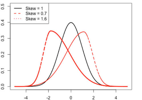
Skewness is an expression of how lopsided a distribution appears. In other words, it measures the asymmetry of a distribution.
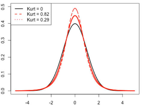
Kurtosis measures the peakedness or flatness of a distribution. In financial return distributions, it describes how fat or skinny the tail is. A fat tail means that a distribution has a larger kurtosis value than a normal distribution. Consequently, more extreme events are likely to be observed.
Over time, people realized that return distributions have some stylized facts. In Economics, stylized facts are empirical discoveries of a phenomenon or observation. People have broadly accepted these stylized facts.
Stylized Facts of Financial Returns
- Fat Tails
- Asymmetry
- Absence of Serial Correlations
- Volatility Clustering
- Time-Varying Cross-Correlations
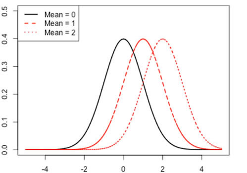
Normal Distribution, Limitations and Alternatives
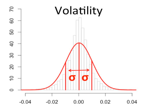
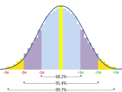 A widely used type of distribution to model financial returns is called
the normal distribution. This model displays a shape known as a Bell
Curve, shown to the right. The premise of the normal distribution is that any
collection of measured amounts (such as blood pressure readings, SAT scores,
batting averages) will tend to form a bell curve around the mean of the
collection; this curve will be defined such that 68.3% of all records will
be graphed within one standard deviation* above (to the right of) or below
(to the left of) the mean of the center line, 95.4% of all records will
be within two standard deviations higher or lower than the mean, and 99.7%
of all records will located on the chart within three standard deviations
from the mean.
A widely used type of distribution to model financial returns is called
the normal distribution. This model displays a shape known as a Bell
Curve, shown to the right. The premise of the normal distribution is that any
collection of measured amounts (such as blood pressure readings, SAT scores,
batting averages) will tend to form a bell curve around the mean of the
collection; this curve will be defined such that 68.3% of all records will
be graphed within one standard deviation* above (to the right of) or below
(to the left of) the mean of the center line, 95.4% of all records will
be within two standard deviations higher or lower than the mean, and 99.7%
of all records will located on the chart within three standard deviations
from the mean.
*Written as "1s", also called "Sigma"; a statistical number representing a specific amount of dispersion from the mean
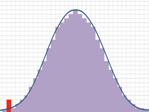 The appeal for use of a normal distribution is that it's easy to calculate,
and it measures central tendency. The weakness is it ignores the extreme
events, also known as outliers or fat-tails. Extreme events occur much
more frequently than estimated in a normal distribution. In the distribution chart to the right the red bar
is a left-tail outlier, it represents an extreme drop in the price of the
security which created a return that is far below the mean for this particular
time period. The table below illustrates the extreme event forecasts under
the normal distribution versus reality.
The appeal for use of a normal distribution is that it's easy to calculate,
and it measures central tendency. The weakness is it ignores the extreme
events, also known as outliers or fat-tails. Extreme events occur much
more frequently than estimated in a normal distribution. In the distribution chart to the right the red bar
is a left-tail outlier, it represents an extreme drop in the price of the
security which created a return that is far below the mean for this particular
time period. The table below illustrates the extreme event forecasts under
the normal distribution versus reality.
| A Loss in this Standard Deviation Range... | Predicted to Occur Every... | Actually Occurs Every... |
|---|---|---|
| 1s | 6 days | 8 days |
| 2s | 44 days | 35 days |
| 3s | 741 days | 137 days |
| 4s | 31,547 days | 484 days |
| 10s | 512.6+ sextillion years | 15,491 days |
The table below represents the normality test on the S&P 500's returns from 1950 to 2012. A normality test, as its name suggests, tests whether a return distribution is normally distributed.
| Test | Jarque-Bera Normality Test |
|---|---|
| Statistics | X-squared: 508881.035 |
| P-value | Asymptotic p value: < 2.2e-16 |
The result from table above rejects the hypothesis that returns are normally distributed. Furthermore, let us do a visual inspection on the non-normality of returns. The tables below are called QQ plots. If most of the actual data (black dots) are within the dashed red lines and there is no massive deviation from the solid red line, we say that the returns of this asset are likely to have a corresponding parametric distribution. Again, S&P 500 returns are used. In this case, let us compare a Normal distribution and a Skew T distribution.
| QQ Plots: S&P 500 1950-01-04 to 2012-12-10 | |
|---|---|
| Normal | Skew T |
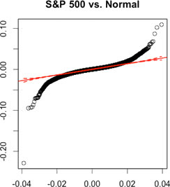 |
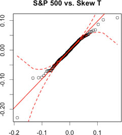 |
| Massive deviations from the solid red line occur on both tails. None of the black dots are within the dashed red lines on both tails. | Fewer deviations from the solid red line occur on both tails. All of the black dots are within the dashed red lines on both tails. |
A normal distribution is not the only model for measuring financial returns. There are several other forms of distributions, including Student-t, Skew T, Stable or mixture distributions. People have discovered other kinds of non-normal distributions that can model skewness (asymmetry) and kurtosis (fat-tails) of financial returns. In other words, certain non-normal distributions capture all four moments of a return distribution at the expense of greater complexity.
Volatility
Definition
 Loosely speaking, volatility is a statistical measure of the dispersion
of returns from its mean for a financial asset. Volatility is often thought
to be the default risk measure in the financial industry. It is also known
as the standard deviation or sigma (s). It is assumed that a higher value for the
standard deviation equates to more risk.
Loosely speaking, volatility is a statistical measure of the dispersion
of returns from its mean for a financial asset. Volatility is often thought
to be the default risk measure in the financial industry. It is also known
as the standard deviation or sigma (s). It is assumed that a higher value for the
standard deviation equates to more risk.
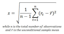
Mathematically, volatility (s) is often measured by the sample statistic (s) defined as:
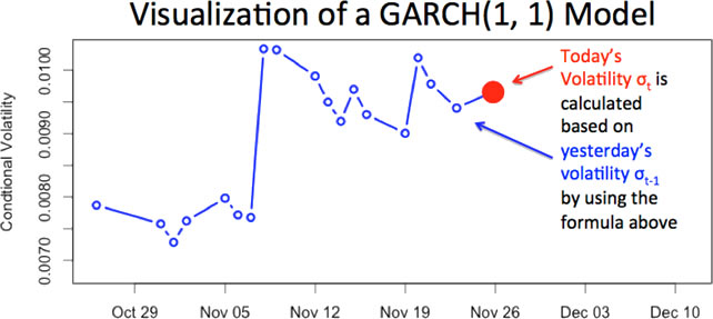
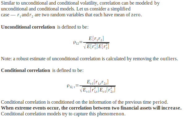
There are two primary ways of describing volatility - conditional and unconditional. Conditional volatility is more responsive to new information than unconditional volatility as shown in the graph below. However, calculating conditional volatility requires more sophisticated mathematics and greater computing power.
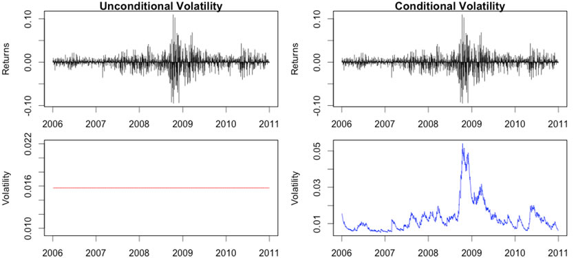
Unconditional modeling of a time series X at time t+1 is based on the unconditional distribution. That is, all statistics are computed from the marginal distribution FX.
Conditional modeling of a time series X at time t+1 is based on the conditional distribution, given some information you can acquire from the previous periods. That is, all statistics are computed from the conditional distribution F(X | It).
Unconditional volatility is the standard deviation of a time series of returns; call that vector, R. Mathematically, it is defined as:
Conditional volatility is conditioned on the information of the previous time period. Therefore it is a process rather than a static number. There are different models, for example, EWMA and GARCH, to model volatility dynamics. Generally speaking, conditional volatility of a time series of returns, R is defined as:
Due to volatility clustering, one of the stylized facts of financial returns,for a short time interval, when volatility is high, it tends to stay high; and when it is low, it tends to stay low. Let us see how a GARCH(1, 1) model captures this phenomenon and how to visualize the actions.
To further show that return series experience ARCH/GARCH effects, we now do a statistical test on S&P 500 from 1950 to 2012.
| Test | ARCH LM-test |
|---|---|
| Statistics | Chi-squared = 1466.152, df = 12 |
| P-value | P-value: < 2.2e-16 |
The result from the table above rejects the hypothesis that there are no ARCH effects in the return series of S&P 500. It confirms our belief that the return series experiences ARCH effects.
Risk Measures Beyond Volatility
Semi-Deviation
Semi-deviation is a measure of downside risk computed as the square root of the average of the variance of the return values below the mean. It is simply the loss side of the distribution. This method was the preferred method of banks and insurance companies for decades, as they had good insight into their revenue side (premiums & deposits).
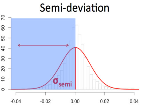
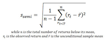
Mathematically, it is defined as:
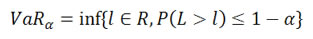
Value-at-Risk (VaR)
Value-at-Risk (VaR) is a threshold value of loss over a given period, often stated with a probability that the loss will exceed this threshold. In other words, 4% VaR at 99% means that you have one percent of chance of experiencing a loss that is at least 4%. VaR has been the current accepted risk measure for the last two decades. In fact, the Bank for International Settlements, under the Basel II Accord, requires VaR as a global risk standard.
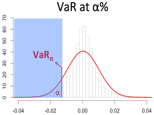
Mathematically, it is defined as:
(Frey and McNeil, 2002) Denote the loss distribution by FL(l)=P(L≤l). Given some confidence level ∝∈(0,1), the VaR∝ is given by the smallest number l such that the probability that the loss L exceeds l is no larger than (1-∝). Formally:
Although VaR measures tail risk and is easy to implement, it has serious limitations. It is only a quantile measure; it tells you nothing about how large losses are beyond VaR. In addition, since VaR is easy to calculate, it is easy to be negligently implemented. Companies can use rudimentary methodologies to calculate VaR to meet investors' risk tolerances. In fact, using simple models, such as a normal distribution, has been deep-rooted in the industry. In portfolio optimization, VaR is a quantile function that is not often smooth, because most return distributions are not normally distributed. This makes it difficult to use VaR in the optimization process.
Expected Shortfall (ES)
Expected Shortfall (ES) also called Expected Tail Loss or Conditional Value-at-Risk, describes the amount of loss to be expected when that loss has breached VaR threshold.
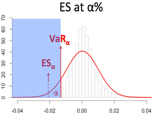
Mathematically, it is defined as:
(Frey and McNeil, 2002) Consider a loss L with continuous density function Fl satisfying ∫R | l | dFL(l) < ∞. Then the Expected Shortfall at confidence level ∝ ∈ (0,1), is defined to be
Perhaps the most attractive property is that expected shortfall is a coherent risk measure that satisfies the four axioms of positive homogeneity, subadditivity, monotonicity and translation invariance. ES has many superior properties compared to volatility, semi-deviation and VaR. Expand below for evidence.
More on Coherent Risk Measure
| Risk Measure | Axiom 1 | Axiom 2 | Axiom 3 | Axiom 4 |
|---|---|---|---|---|
| Volatility | Yes | |||
| Semi-deviation | Yes | |||
| VaR | Yes | Yes | Yes | |
| ES | Yes | Yes | Yes | Yes |
(Artzner, Delbaen, Eber and Heath, 1998) Any coherent risk measure ?: X?R must satisfy the following four axioms:
- Positive homogeneity: ρ(λx) = λρ(x) for all x ∈ X and λ≥0
(Addressing liquidity concerns) - Subadditivity: For all x and y ∈ X, ρ(x+y) ≤ ρ(x) + ρ(y)
(Diversification does not create extra risk) - Monotonicity: For all x and y ∈ ℝ with x ≤ y, we have ρ(x) ≤ ρ(y)
(Semi-deviation type risk measures are ruled out) - Translation invariance: For all x ∈ X and all real number α, we have ρ(x+α⋅r) = ρ(x)-α
(Adding a risk-free return to a random return can reduce risk)
Risk-Reward Measures
Definition
Risk-reward measures distill an asset's performance into a single number to make balancing risk and return more convenient; the higher the risk-reward the more efficient the performance. This section examines absolute risk-reward measures, which use calculations not dependent on any benchmarks. They also serve as objective functions in portfolio optimization. A proper risk-reward measure should accurately reward positive returns and punish excessive risks, hence they are often thought of as risk-adjusted returns.
Sharp Ratio
Sharpe Ratio is the most popular risk-reward measure, and is indeed the default risk-reward measure throughout the industry. Taking the average return of an asset during a period, subtracting the risk-free rate and dividing it by its standard deviation is how you calculate Sharpe Ratio.
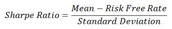
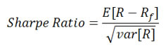
Although Sharpe Ratio is widely accepted as the default risk-reward measure, it has some fundamental flaws. Using volatility (standard deviation) to quantify risk, it thus implicitly assumes a Normal distribution for returns, which underestimates tail risk. While volatility is not always bad, Sharpe Ratio punishes "good volatility" as well as "bad volatility". The standard industry method of calculating Sharpe Ratio is still unconditional modeling, so it doesn't reflect any real-time performance. This leads to untimely decisions that could potentially be costly mistakes. Lastly, volatility is not a coherent risk measure.
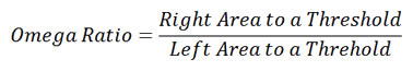
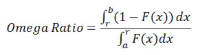
Omega Ratio
Omega Ratio is an alternative to the Sharpe Ratio. It does not assume returns are normally distributed; and it doesn't depend on the choice of distributions. In short, the Omega Ratio measures the probability of good versus bad returns. Given any return distribution, it is calculated by dividing the area to the right of a given threshold value by the area to the left of this value.
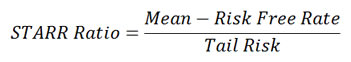
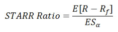
STARR Ratio
STARR Ratio (Stable Tail Adjusted Return Ratio) replaces volatility with expected shortfall as the coherent risk measure. Unlike the Sharpe Ratio, STARR Ratio only penalizes downside tail-risk of an asset instead of volatility. Skewness and fat-tails can be measured with STARR.
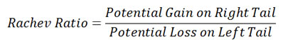
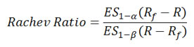
Rachev Ratio
Rachev Ratio is the ratio between the expected shortfall of the excess return at a given confidence level 1-a and the expected shortfall of the excess return at another confidence level 1-b.
Dependence Measures
Definition
In finance, it is common to study multiple securities at the same time. This makes it critical to understand how assets move together which can be quantified with dependence measures. In statistics, the correlation coefficient measures the statistical relationships between variables. Familiar examples include summer temperature and ice cream consumption, stock price of a gold mining company and gold price, etc. Here are some notes worth attention:
- The term "correlation" in finance, often refers to Pearson's correlation coefficient which measures linear relationships of variables. However, there are many types of correlation coefficients (for example, rank correlation, distance correlation, etc.).
- The relationships between two variables can be positive or negative, linear or non-linear. In finance, the relationships between two securities often cannot be completely characterized by a linear correlation, especially during crisis periods.
- Correlation does not imply causation. For example, the price of a candy bar might be positively correlated to the crime rate of a city, but there is no obvious and reasonable causation between those two events.
Linear Relationship
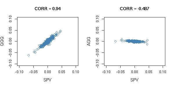
Pearson's product-moment correlation coefficient (often referred to as "Pearson's r" or simply "correlation") is a measure of the linear correlation between variables. Pearson's r has a value ranging from +1 to -1. A positive value indicates a positive linear relationship between two variables and vice versa. For example, from June 1st, 2011 to December 31st, 2012 SPY and QQQ are both ETFs based on US equity indices. Therefore, historically, their daily returns have a positive Pearson's r of 0.94. In contrast, SPY and AGG are historically negatively correlated. Therefore a negative Pearson's r of -0.487 is observed.
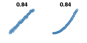
Correlation, specifically Pearson's r, is thought to be the default measure of relationships in the financial industry. However, it has some weaknesses. The most well-known is that Pearson's r fails to see non-linear relationships which are often observed in reality. Below is a simplified example of a non-linear relationship, both have Pearson's r values of 0.84, but we can see that there is an obvious non-linear relationship for the graph on the right. Another shortcoming of Pearson's r is that there are several assumptions which may or may not always be realistic. For example, for Pearson's r to work well, financial returns must be normally distributed. Another shortcoming is that Pearson's r does not measure the magnitude of co-movement of variables. This phenomenon is called concordance. For more rigorous explanations on the shortcomings of Pearson's r, please review the Mathematical Definition below.
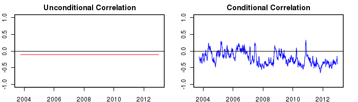
There are two primary ways of describing correlation: conditional and unconditional. Conditional correlation is more responsive to new information than unconditional correlation as shown in the graph below. However, calculating conditional correlation requires more sophisticated mathematics and greater computing power. The example below is the unconditional and the conditional correlation between SPY and AGG from September 30th, 2003 to December 12th, 2012.
Non-Linear Relationship
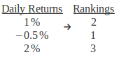
A ranking is a relative position in a group. For example, we have three daily returns; their rankings are demonstrated in the table below:
Instead of working with the actual variables, a rank correlation coefficient measures the relationships between rankings of the underlying variables. Common rank correlation coefficients includes Spearman's rho rank correlation coefficient (also known as "Spearman's rho") and Kendall's tau rank correlation coefficient (also known as "Kendall's tau' or "t".) Similar to the linear correlation, Pearson's r, both Spearman's rho and Kendall's tau measure the linear relationship between two variables. However, due to the advantage of working with the rankings instead of the actual variables, Spearman's rho and Kendall's tau may also capture non-linear relationships.
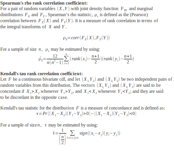
Unlike linear correlation, Pearson's r, Spearman's rho and Kendall's tau don't share the same shortcomings of Pearson's r. They can measure non-linear relationships of financial security returns; they are very versatile with few assumptions. In addition, they measure concordance.
Dependency Structure
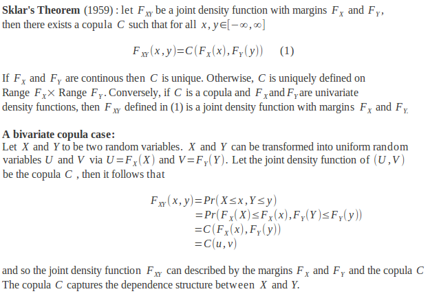
Since the birth of Modern Portfolio Theory, using linear correlation, Pearson's r, to capture co-movement between financial asset returns has been the standard approach. Relationships may in reality be linear or non-linear. An alternative approach to measure dependence is to use copulas.
In linguistics, the word copula derives from the Latin noun for a "link" or "tie" that connects two different things. In finance, copulas model the "links" between different financial assets. The theory of copulas provides a flexible methodology to model non-linear relationships without unrealistic assumptions on individual financial assets. There are many types of copulas, each with different advantages and disadvantages. One potential advantage, using a t-copula, is the ability to model tail dependence, which is an increase in correlation during extreme scenarios. A Gaussian copula, used extensively in finance during 2008, does not share this advantage.
Copulas, despite of their misusage, are definitely a breakthrough in modern finance. It has become the most significant new technique to handle co-movement between markets and risk factors in a flexible way. Criteria for selecting a copula model may include non-linear relationships, tail dependency, time-varying or regime switching features, computational and estimation efficiency. The ongoing efforts of copula modeling may include vine structures, regime switching models, conditional models and more.
Allocation Methodologies
Definition
Allocation Methodologies are sets of rules which govern the percentage weight of each individual asset within a portfolio of multiple assets. The total percentage weights when added together will equal 100%. In practice, ignoring short positions, the percentage weights can range from 0% to 100%. The set of rules to select percentage weights, or allocation weights, can be simple, highly complex or variations in between.
Several methodologies approach this problem by aiming to balance risk and reward according to an investor's goals, risk tolerance and time horizon. Different asset classes, for example, equities, fixed income and commodities, have different levels of risk and return and may have different merits for inclusion/exclusion from an investor's final allocation weightings.
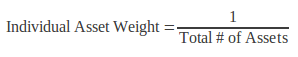
Equal Weighting (EQW)
Equal Weighting (EQW) is one example of an asset allocation methodology that is relatively simple to apply. As the name suggests the rule states to hold an equal percentage weight of each individual asset. The benefits of this approach are that no single position will be too large and the method is simple to compute and apply. The limitations include ignoring any risk or return information, nor does it consider how assets move in relation to one another.
Modern Portfolio Theory (MPT)
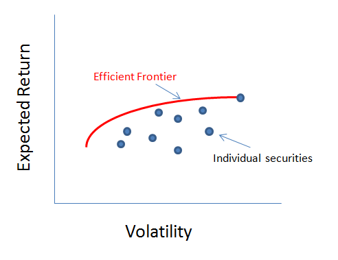
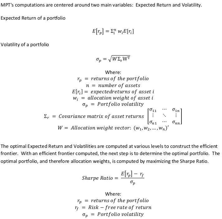
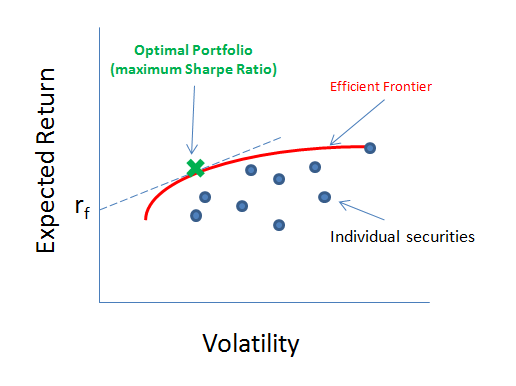
Modern Portfolio Theory (MPT) has historically been the industry standard for allocation methodologies. Developed in 1952 by Harry Markowitz, this method explains how a risk-averse investor can decide allocation weights to maximize reward based on a given level of risk. Reward is expressed as expected return and risk is expresed as volatility of the portfolio. The ratio of these is called the Sharpe Ratio. This is then defined as the optimal portfolio. In general, to obtain higher levels of reward, an investor has to take on higher levels of risk. Based on Markowitz's theory, it becomes possible to compute an "efficient frontier" which is a set of optimal portfolios which provide the lowest level of risk for any given expected return.
The advantages of MPT include the following: a method to balance risk and reward, accounts for inter-market relationships, and it's simple to compute. The limitations of this approach include an implicit assumption of the normality of asset returns. This may underestimate risk in certain market environments. Additionally, the inter-market relationships are based on linear-correlation which may not always be appropriate.
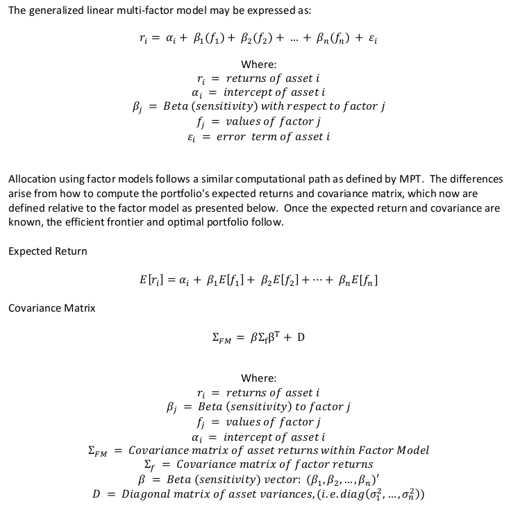
Factor Models
Factor Models are mathematical descriptions which explain an individual asset's returns. These models can be quite useful in allocation methodologies. Factors which help explain an asset's return can be of several types. Examples would be economic indicators (e.g. unemployment and industrial production) or fundamental factors (e.g. earnings and valuation metrics). The benefits of using this approach include a better understanding of an asset's sources of risk and an improved understanding of the relationship between the assets. The limitations include the complexity and difficulty of identifying explanatory factors and relationships. There also exist some of the same limitations within MPT. For example, an implicit assumption of normality of returns which may underestimate risk and a reliance on linear relationships which may not reflect complexities in assets' relationships.
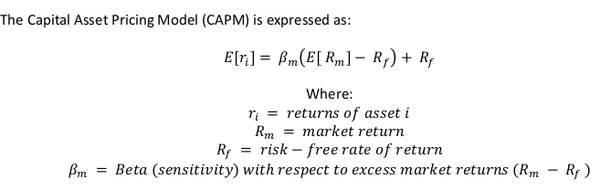
Capital Asset Pricing Model (CAPM)
Capital Asset Pricing Model (CAPM) is one of the earliest examples of a factor model in use in the finance industry. This model uses a single factor, excess market returns, to predict an asset's return. Excess market returns are also thought of as non-diversifiable risk (a.k.a. systematic risk or market risk).
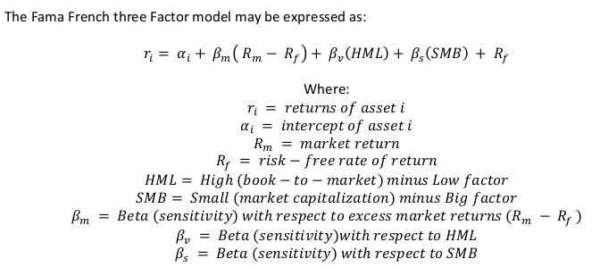
Fama French Factor Model (FF)
Fama French Factor Model (FF) is a specific type of factor model which uses three factors to explain asset returns. Those factors are excess returns on the market, size of firms and book-to-market values. Developed in the early 1990's by Eugene Fama and Kenneth French, this model expands on the single factor CAPM. The two professors noted that two groups of stocks typically outperformed the overall stock market. The first group is small cap stocks which are firms of a smaller size as measured by market capitalization. The second group is value stocks which are stocks with a high book-to-market ratio, or alternatively stated, a low price-to-book ratio. They identified two factors to account for these phenomena and added the factors to CAPM. The intended result is to gain a better explanation of individual asset returns relative to CAPM.
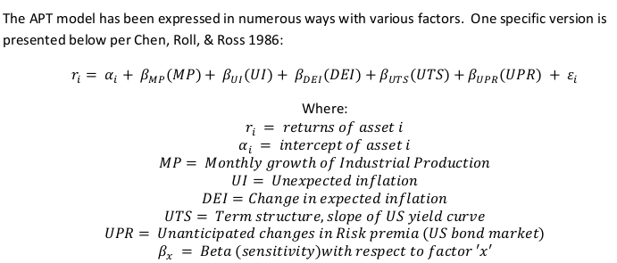
Arbitrage Pricing Theory (APT)
Arbitrage Pricing Theory (APT) is a set of factor models. They were initially proposed by economist Stephen Ross in 1976 in which the factors are macro-economic or theoretical market indices. Specific examples of APT factors include: unexpected inflation, industrial production, etc. In APT, the expected return of an individual asset is modeled based on these factors and consequently the asset may be priced theoretically. When the current actual market price deviates from the model's theoretical price, APT suggests arbitrage will bring the prices back into agreement.
Dynamic Portoflio Optimization (DPO)
Dynamic Portfolio Optimization (DPO). The aforementioned allocation methods, MPT, CAPM, APT and Fama French, rest upon several implicit assumptions. Those are normality in return distributions, a static measure of risk and linear inter-market relationships which may oversimplify how markets interact. While the specific details of this methodology are proprietary, the results of DPO are allocation weights that reflect real-time risk-reward characteristics of assets within a portfolio. The limitation of using DPO is its computational complexity.
Allocation Methodology Comparison
Allocation Methodology Comparison
| Equal Weighting | MPT | APT | Fama French | DPO | |
|---|---|---|---|---|---|
| Distribution Assumption | N/A | Normality | Normality | Normality | No Assumption |
| Time-varying Risk | No | No | No | No | Yes |
| Relationship Model | None | Linear Correlation | Linear Correlation within Factor structure | Linear Correlation within Factor structure | Non-linear |
References
Artzner, Philippe, Freddy Delbaen, Jean-Marc Eber, and David Heath. "Conerent
Measures of Risk." (July 22, 1998).
www.math.ethz.ch/~delbaen/ftp/preprints/CoherentMF.pdf
Chen, Nai-Fu, Richard Roll, and Stephen A. Ross. "Economic Forces and
the Stock Market." (July 1986).
rady.ucsd.edu/faculty/directory/valkanov/pub/classes/mfe/docs/ChenRollRoss_JB_1986.pdf
Engle, Robert. "Dynamic Conditional Correlation - a Simple Class of Multivariate
GARCH Models." (July 1999).
weber.ucsd.edu/~mbacci/engle/391.PDF
Frey, Rudiger, and Alexander J. McNeil. "VaR and Expected Shortfall in
Portfolios of Dependent Credit Risks: Conceptual and Practical Insights."
(January 23, 2002).
www.mathematik.uni-leipzig.de/~frey/rome.pdf
Fama, F. Eugene, and Kenneth R. French. "Common Risk Factors in the Returns
on Stocks and Bonds." (September 1992).
home.business.utah.edu/finmll/fin787/papers/FF1993.pdf
Fama, F. Eugene, and Kenneth R. French. "The Cross-Section of Expected
Stock Returns." (June 1992).
www.bengrahaminvesting.ca/Research/Papers/French/The_Cross-Section_of_Expected_Stock_Returns.pdf
Markowitz, Harry. "Portfolio Selection: Efficient Diversification of Investments." (1959).
Ruppert, David. Statistics and Data Analysis for Financial Engineering Statistics and Data Analysis for Financial Engineering. Ithaca: Springer, 2010.
Ross, A. Stephen. "The Arbitrage Theory of Capital Asset Pricing." (May
19, 1976).
www3.nccu.edu.tw/~cclu/FinTheory/Papers/Ross76.pdf
Sharpe, F. William. "Capital Asset Prices: A Theory of Market Equilibrium
under Conditions of Risk." (September 1964).
onlinelibrary.wiley.com/doi/10.1111/j.1540-6261.1964.tb02865.x/pdf
Zivot, Eric. "Financial Econometrics and Quantitative Risk Management."
(May 29, 2013).
faculty.washington.edu/ezivot/econ589/estimatingmacrofactormodels.pdf